Retrospective Analysis
Source:vignettes/articles/Retrospective-Analysis.Rmd
Retrospective-Analysis.RmdRetrospective analysis is commonly used to check the consistency of
model estimates such as spawning stock biomass (SSB) and fishing
mortality (F) as the model is updated with new data. The retrospective
analysis involves sequentially removing observations from the terminal
year (i.e., peels), fitting the model to the truncated series, and then
comparing the relative difference between model estimates from the
full-time series with the truncated time-series. To implement a
retrospective analysis with Stock Synthesis the r4ss
package provides the retro() function. Here we provide a
step-by-step example of how to run and interpret a retrospective
analysis using a simple SS model.
Model inputs
To run a stock synthesis model, 4 input files are required:
starter.ss, forecast.ss, control.ss, and data.ss. The input files for
the example model can be found within the ss3diags package
and accessed as shown below. Also, if you do not have the
r4ss package installed, you will need to install it for
this tutorial.
install.packages("pak")
pak::pkg_install("r4ss/r4ss")
library(r4ss)

files_path <- system.file("extdata", package = "ss3diags")
dir_retro <- file.path(tempdir(check = TRUE), "retrospectives")
dir.create(dir_retro, showWarnings = FALSE)
list.files(files_path)
#> [1] "control.ss"  "data.ss"     "forecast.ss" "starter.ss"
file.copy(from = list.files(files_path, full.names = TRUE), to = dir_retro)
#> [1] TRUE TRUE TRUE TRUE
You will need to make sure you have the SS
executable file either in your path or in the directory you are
running the retrospective from (in this case dir_retro). An
easy way to get the latest release of stock synthesis is to use the
r4ss function get_ss3_exe().
r4ss::get_ss3_exe(dir = dir_retro, version = "v3.30.21")
#> The stock synthesis executable for Linux v3.30.21 was downloaded to: /tmp/RtmpLEkSvl/retrospectives/ss3
Retrospective Analysis
Once you have the 4 input files and the SS executable file, you can
run a retrospective analysis as shown below. We are running it for five
one-year peels, so with each run, one to five years of data are removed
from the reference model and the model is re-run for a total of five
times (i.e. peel 1 removes the last year of data, peel 2 removes the
last 2 years of data, etc.) . The number of year peels can be adjusted
with the years argument. If the SS executable file you are
using is named something other than “ss3” (e.g. ss_opt_win.exe), you
will need to specify this with the argument
exe = "ss_opt_win". Full documentation of the
retro() function can be found on the r4ss
website.
r4ss::retro(dir = dir_retro, exe = "ss3", years = 0:-5, verbose = FALSE)
#> Warning in base::sink(type = "output", split = FALSE): no sink to remove
Visualizing Output
To visualize the outputted results and inspect them for any
retrospective patterns, you will need to load the report files into R
and use the SSplotRetro() function from
ss3diags. The easiest way to load multiple report files is
using r4ss::SSgetoutput() and
r4ss::SSsummarize() functions. The default sub-directories
for each peel, 0 to 5, are labeled retro0 to
retro-5.
retro_mods <- r4ss::SSgetoutput(dirvec = file.path(dir_retro, "retrospectives", paste0("retro", seq(0, -5, by = -1))), verbose = F)
retroSummary <- r4ss::SSsummarize(retro_mods, verbose = F)
SSplotRetro(retroSummary, subplots = "SSB", add = TRUE)
#> Mohn's Rho stats, including one step ahead forecasts:
#>   type     peel         Rho  ForecastRho
#> 1  SSB     2021 -0.20753686 -0.221050163
#> 2  SSB     2020 -0.19601072 -0.227304734
#> 3  SSB     2019 -0.29238505 -0.338600758
#> 4  SSB     2018 -0.00474920 -0.007462034
#> 5  SSB     2017  0.08716428  0.098849082
#> 6  SSB Combined -0.12270351 -0.139113722
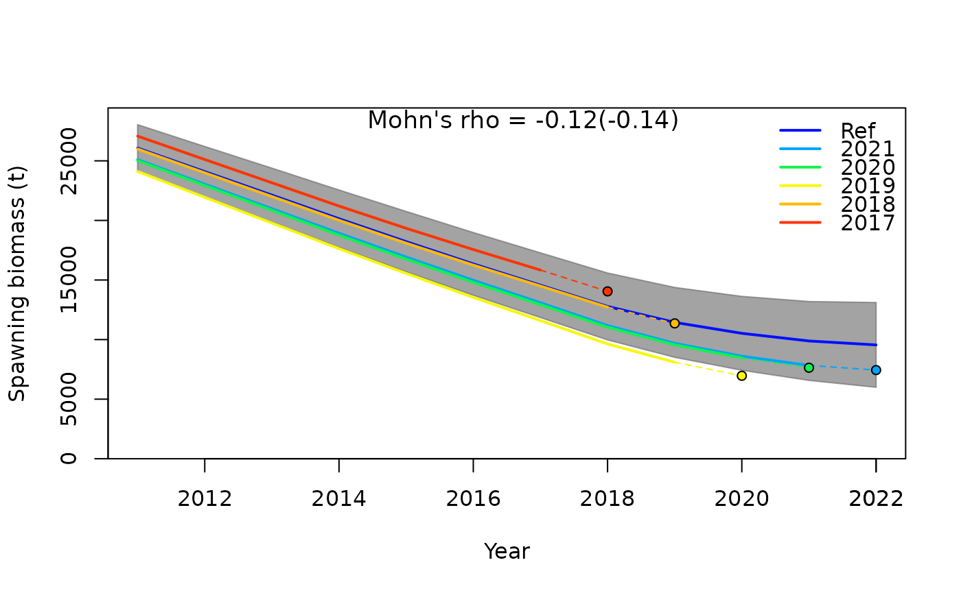
The default settings plot the spawning stock biomass time series for
each peel, with the reference run (i.e. original, full time series
model) as the “Ref” line and each successive peel as colored lines
labeled by their terminal year value. The solid line ends at the
terminal year followed by the dashed line extending to a circle
representing the one year forecast estimate. Displaying the projected
SSB value helps in assessing forecast bias. Of note, forecasts are done
automatically when using r4ss::retro() and are based on the
settings in forecast.ss. The grey shaded area represents the 95%
confidence intervals of uncertainty around the spawning biomass time
series. Displayed in the center of the plot is the combined Mohn’s
for all retrospective runs, and in parentheses is the forecast Mohn’s
.
Customizing the Plot
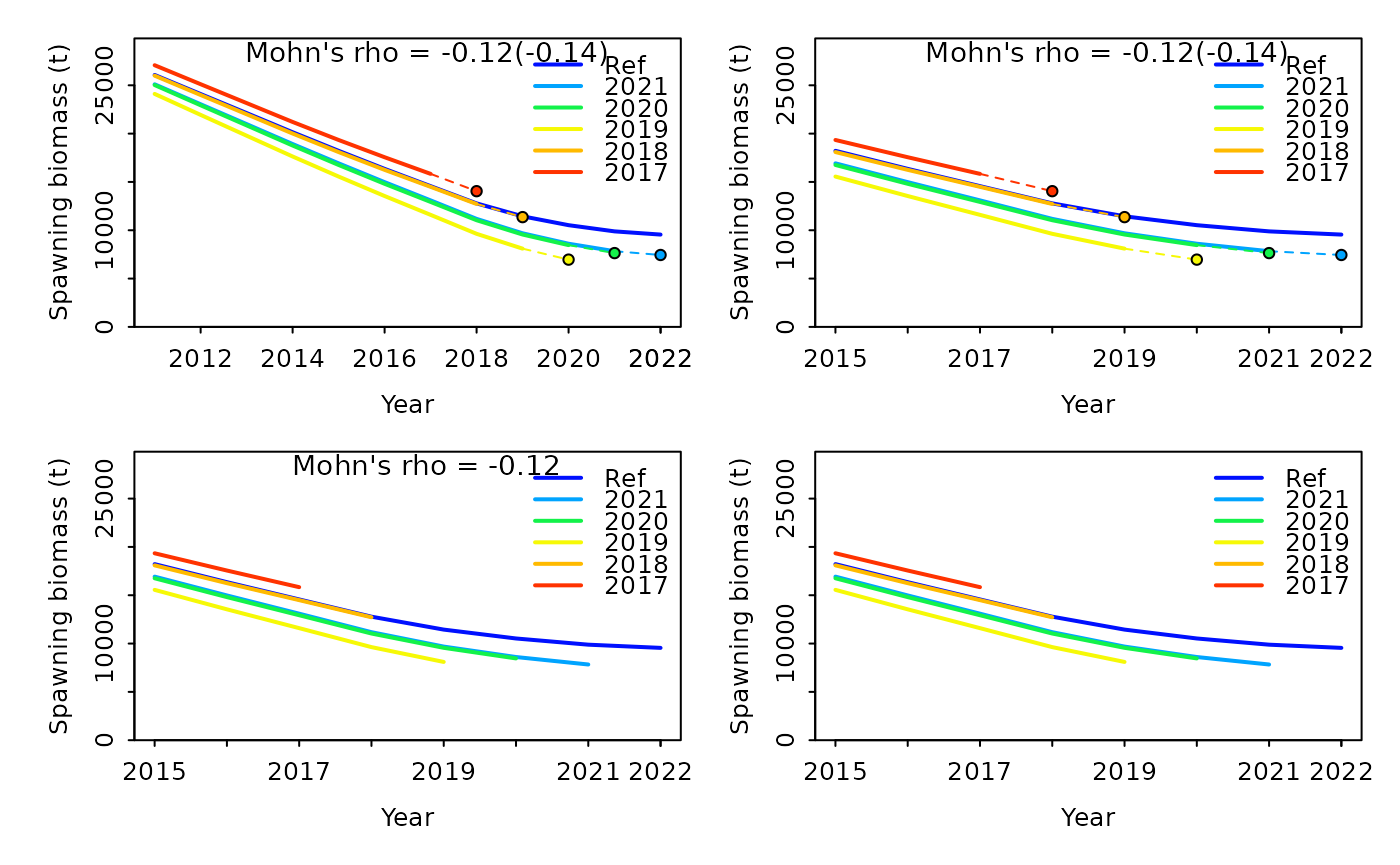
Retro plots can be customized in many ways, some common features that you may want to specify are:
- removing uncertainty intervals
- adjusting the years shown on the x-axis
- turning off the 1-year ahead forecasting
- not displaying the combined value on the plot
Examples of each of these changes are shown below, incrementally making each adjustment.
r4ss::sspar(mfrow = c(2, 2), plot.cex = 0.8)
retro1 <- SSplotRetro(retroSummary, subplots = "SSB", add = TRUE, uncertainty = FALSE)
#> Mohn's Rho stats, including one step ahead forecasts:
retro2 <- SSplotRetro(retroSummary, subplots = "SSB", add = TRUE, uncertainty = FALSE, xlim = c(2015, 2022))
#> Mohn's Rho stats, including one step ahead forecasts:
retro3 <- SSplotRetro(retroSummary, subplots = "SSB", add = TRUE, uncertainty = FALSE, xlim = c(2015, 2022), forecast = FALSE)
#> Mohn's Rho stats, including one step ahead forecasts:
retro4 <- SSplotRetro(retroSummary, subplots = "SSB", add = TRUE, uncertainty = FALSE, xlim = c(2015, 2022), forecast = FALSE, showrho = FALSE, forecastrho = FALSE)
#> Mohn's Rho stats, including one step ahead forecasts:Additionally, fishing mortality can be plotted instead of spawning
biomass by replacing subplots = "SSB" with
subplots = "F"
Summary Table
In addition to the retrospective plots, a summary statistics table
can be produced using SShcbias(). This table includes
- type of estimate (SSB or F)
- the year removed or “peel”
- Mohn’s
- forecast bias
by year and overall (“Combined”). Mohn’s is a measure of the severity of bias in the retrospective patterns and the forecast bias is an estimate of bias in the forecasted quantities when years of data were removed. The rule of thumb proposed by Hurtado-Ferror et al. (2014) for Mohn’s values is that for long-lived species, the value should fall between -0.15 and 0.20.
SShcbias(retroSummary)
#> Mohn's Rho stats, including one step ahead forecasts:
#>    type     peel         Rho   ForcastRho
#> 1   SSB     2021 -0.20753686 -0.221050163
#> 2   SSB     2020 -0.19601072 -0.227304734
#> 3   SSB     2019 -0.29238505 -0.338600758
#> 4   SSB     2018 -0.00474920 -0.007462034
#> 5   SSB     2017  0.08716428  0.098849082
#> 6   SSB Combined -0.12270351 -0.139113722
#> 7     F     2021  0.28425747  0.285936183
#> 8     F     2020  0.30941305  0.349748774
#> 9     F     2019  0.52629045  0.632574831
#> 10    F     2018  0.01822898  0.022822958
#> 11    F     2017 -0.04896989 -0.053882358
#> 12    F Combined  0.21784401  0.247440078